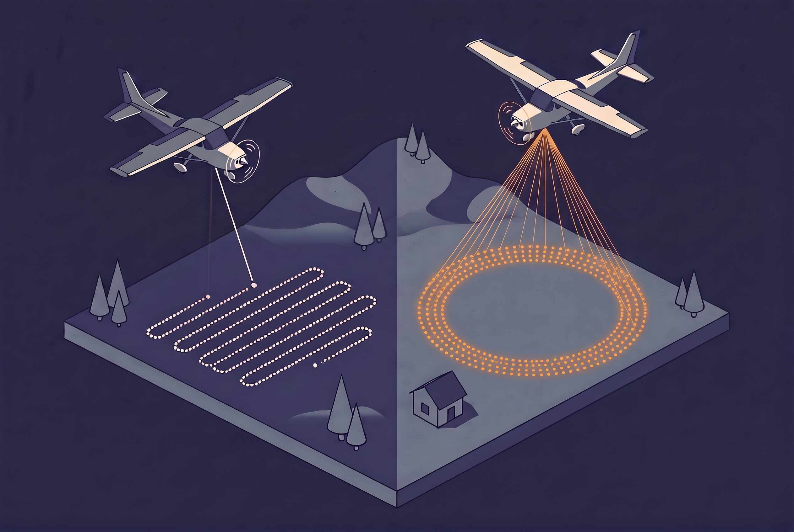
In Navarre, Spain, the mapping agency Tracasa flew the same region of about 10,400 square kilometers twice. The first campaign, flown in 2011 and 2012 with a linear-mode LiDAR sensor, took about 270 flight hours and produced 1.2 points per square meter. The second used a single-photon sensor, took about 170 hours, and averaged 14 points per square meter. According to a customer story published by Leica Geosystems, that is roughly twelve times the density in about 100 fewer flight hours.
Results like that explain the attention single-photon LiDAR (SPL) has received since the first commercial sensor appeared in 2017. They also raise an obvious question: if one sensor collects this much more data per flight hour, why are airborne surveys not all flown this way? The answer combines physics and market structure. SPL trades some precision and data cleanliness for its productivity, and as of October 2026 it remains a niche technology with one main supplier. This article explains how SPL differs from linear-mode LiDAR, what independent testing shows about the trade-offs, and how far adoption has actually gone.
Linear-Mode LiDAR in Brief
Most airborne LiDAR collected today is linear mode, a name that comes from the way the detector responds: its output grows in proportion to the amount of light that hits it. The system fires a laser pulse, and the light returning from the ground, a roof, or a branch is converted into an electrical signal. That signal is proportional to the number of photons that arrived. To measure a range reliably, the detector needs a signal clearly above its noise floor, which in practice means hundreds of photons per return.
Two things follow from that requirement. The sensor needs a strong laser pulse and a detector that is sensitive but not extreme, typically an avalanche photodiode working in the near-infrared. And because each pulse carries so much energy, the pulse repetition rate is limited, to roughly 1 to 2 million pulses per second in current Leica systems. A single pulse can still produce several returns, such as the top of a tree, a branch in the middle of the canopy, and the ground. Most modern linear-mode sensors record these as discrete returns, and some also record the full waveform.
The approach is mature and well understood. Its cost is efficiency. To collect enough photons, linear-mode systems fly relatively low and slow, and covering a large area takes many flight lines. That ties the technology directly to survey altitude and to the price of every flight hour, which is exactly the part of the equation that SPL attacks.
How Single-Photon LiDAR Works
SPL reverses the linear-mode trade-off. Instead of firing a strong pulse and waiting for many photons to return, it uses a detector array sensitive enough to register a single arriving photon. With that sensitivity, a modest laser can be split into many beams, and each beam still produces a usable range measurement.
The Leica SPL100 shows the idea clearly. According to Dr. A. Stewart Walker in LIDAR Magazine, a single 5 W laser is split into 100 beams, which gives an effective pulse rate of 6 MHz. The same article lists the linear-mode Leica TerrainMapper at 2 MHz from a 20 W laser, so SPL delivers three times the pulse rate from one quarter of the laser power.
Several other design choices set SPL apart. The SPL100 works with green light at 532 nm, partly for historical reasons tied to early detector arrays, and green light can also penetrate shallow, clear water. Its pulses can be as short as 100 picoseconds, compared with roughly 3 nanoseconds in linear-mode systems such as the ALS80. Each beam behaves like a small linear-mode channel of its own, which is why the article compares the SPL100 to 100 linear-mode systems working in parallel. Targets about 24 cm apart in range can be separated, which helps with low brush and with ground under vegetation.
Single-Photon and Geiger-Mode LiDAR
SPL is often lumped together with Geiger-mode LiDAR because both use detector arrays that respond to single photons. The two approaches differ in what happens after a photon arrives, and that difference shapes how each system collects data.
Geiger-mode detectors register only one return per pixel per pulse, as Ron Roth, a former Hexagon product manager and a former colleague of mine, explained in the same LIDAR Magazine article. They also detect only a small share of the available photons, perhaps 35 percent or less, so a single pulse tells you very little. To compensate, Geiger-mode systems fire many pulses at the same spot. Because real surfaces create returns at a consistent range across many pulses, they can be distinguished from the random returns caused by noise. 3DEO is one vendor in this space, and LIDAR Magazine profiled the company in late 2024.
SPL treats each pulse differently. It behaves more like an array of linear-mode channels, so a single pulse can record multiple returns, for example from a tree canopy and the ground beneath it. The detector is still sensitive to single photons, but the system does not depend on piling up repeated samples to find the signal in the same way. If you know linear-mode LiDAR, SPL is the closer mental model, just with many more channels looking at once. SPL also has a spaceflight pedigree. The Sigma Space team that built the early airborne instruments developed timing electronics for NASA’s ICESat-2 mission, which launched in September 2018. Hexagon acquired Sigma Space in early 2016 and turned its prototype into the commercial SPL100.
What Changes in Practice
The headline difference is productivity. SPL collects far more measurements per second from a smaller laser, which allows higher altitude, wider swaths, and fewer flight lines for the same point density. The table compares the published figures for Leica’s linear-mode and single-photon systems.
| Property | Linear mode (Leica TerrainMapper) | Single photon (Leica SPL100) | Newer SPL module (announced 2024) |
|---|---|---|---|
| Effective pulse rate | 2 MHz | 6 MHz | Over 14 MHz |
| Laser power | 20 W | 5 W | Not stated |
| Output beams | 1 | 100 channels | 500+ channels |
| Field of view | 20-40 degrees | Up to 30 degrees | 60 degrees |
| Typical point density | 10-50 pts/m2, depending on altitude | 12 to 30 pts/m2, depending on altitude | Not stated |
The figures come from LIDAR Magazine, the Leica SPL100 product page, the Hexagon press release, and GeoWeek News. Vendor claims for the size of the gain vary. Leica markets the SPL100 as up to 10 times more efficient than conventional sensors. Ron Roth, the former Hexagon product manager quoted in LIDAR Magazine, was more careful and put productivity at a minimum of 3 times and more likely 6 to 10 times that of linear mode. The newer module is described as a more than fivefold increase in collection rate over traditional linear mode. These are vendor statements, and the spread between them is a reminder that the gain depends on the project.
The Navarre project from the opening is the clearest real-world data point, and it needs two cautions. The earlier campaign used a Leica ALS60, an older generation than the TerrainMapper, so some of the gain reflects a decade of general progress. The figures also come from Leica’s own publication, which states an accuracy better than 20 cm horizontally and 15 cm vertically for the SPL100 data. Even so, the result matches the pattern SPL promises: much denser data in noticeably less flying time, which is what the efficiency of an aerial survey comes down to.
What Independent Testing Shows
Single-photon sensitivity buys speed and density. It costs precision, cleanliness, and detail inside the canopy. A rigorous independent test of the SPL100 is a 2020 study by Rebecca Brown, Preston Hartzell, and Craig Glennie of the University of Houston, published in Remote Sensing. They compared the SPL100 with a linear-mode Optech Titan over the same campus. The table shows the results that matter most for the trade-off. Note that the two sensors flew at very different heights, as is typical for each technology. The study did not test acquisition efficiency, the main selling point of SPL, and it reports no flight times.
| Metric (University of Houston test) | Linear mode (Optech Titan, 532 nm channel) | Single photon (Leica SPL100) |
|---|---|---|
| Flying height above ground | 500 m | 3,700 m |
| Planar ranging scatter, all samples | 1.2 cm | 3.2 cm |
| Pulses with multiple returns in canopy | 87% | 22% |
| Pulses reaching the ground in canopy | 71% | 43% |
| Ground point density under canopy | About 10 points per square meter | About 28 points per square meter |
The first lesson concerns precision. Each SPL range comes from only a few photons, so the system cannot model the shape of a returning pulse the way a linear-mode detector can. The authors found that precision suffered more on dark surfaces and at steep incidence angles. On flat, open urban terrain, the overall positional accuracy against GNSS checkpoints was still comparable to linear mode.
The second lesson concerns noise, which is built into the technique. Raw SPL point clouds contain false returns from sunlight and from detector dark counts, so they need heavy filtering. A Swedish forestry study in Remote Sensing notes that 532 nm sits close to the peak of solar radiation, which makes the system sensitive to solar noise. Filtering has a price too. In the Houston data, the filter that removes noise also removed many genuine returns inside the canopy. Unfiltered data separated first and second returns by about 4.0 meters, similar to linear mode, while the filtered data separated them by about 10 meters. Although, filtering algorithms have likely improved since then.
Canopy performance depends on how you measure it. SPL reached the ground less often per pulse, yet it still delivered more ground points under trees because it fires so many more pulses. The authors point out that a linear-mode sensor sampled at the same rate would beat SPL on under-canopy density. That is a useful reminder that ground coverage under vegetation depends on more than the number of points collected.
Two practical costs complete the picture. Data volumes are large, and Woolpert’s experience mapping Hawaii highlighted storage demands and longer processing times. The green laser can map shallow, clear water, but it can also blur where the water surface ends, so hydrologic features may need a separate workflow.
The Houston authors concluded that the SPL100 is likely best suited to applications where collection efficiency matters more than maximum accuracy and precision, and they noted that the noise filter makes it less suited to forestry work in its current state. The study used 2017 data and early HxMap processing, and the authors showed that reprocessing with newer software already improved results, so treat the numbers as a snapshot rather than a verdict.
Further reading
- Evaluation of SPL100 Single Photon Lidar Data | Remote Sensing
An independent comparison by Brown, Hartzell, and Glennie of the SPL100 with a linear-mode sensor over the same campus. - Sigma Space Brings Single-Photon to Hexagon | LIDAR Magazine
Dr. A. Stewart Walker on how the technology reached Hexagon, with Ron Roth, a former Hexagon product manager, explaining how SPL differs from linear mode and Geiger-mode. - Pioneering Single Photon LiDAR in Europe | Leica Geosystems Reporter
The customer story on the Navarre campaign, with flight hours and point density compared with the earlier linear-mode survey. - Single Photon Lidar: Benefits and Challenges in Hawaii Mapping | Lidar News
Woolpert’s account of flying SPL in Hawaii, including the storage and processing costs.
How Far Adoption Has Gone
Adoption has been real but narrow. SPL has moved from NASA-linked research to a handful of large commercial projects, and at the end of 2024 LIDAR Magazine counted at least eight SPL100 units in use. The timeline traces the milestones I could verify, oldest first.
Sources for the milestones: LIDAR Magazine, Leica Geosystems, Hexagon, Lidar News, and Remote Sensing.
Three patterns stand out when reading across these sources. The first is that the supply side is narrow. As of today, Hexagon is the only supplier of commercial single-photon airborne sensors. Geiger-mode, the other photon-counting approach, has its own vendors, but it is a different technique with a different data character.
The second is that large-area contracts and content programs drive demand. The earliest sales pitch was the lowest cost per data point for work at state and country scale, and the projects in the timeline match that profile. Navarre sits inside Spain’s national orthophoto program, although I found no evidence that the national LiDAR programs of Europe as a whole moved to SPL. Ontario’s forest inventory, covered in the next section, is the largest program of this kind I found.
The third is that the next generation is still ramping up. The 2024 announcement promised commercial availability in 2025, yet at Intergeo 2025 the sensor was still described as in testing. As of October 2026, I could not find a confirmed delivery or a first project report for the new sensor, so treat its field performance as unproven.
Further reading
- Intergeo 2025 – a Retrospective | LIDAR Magazine
Describes Hexagon’s second-generation single-photon sensor as it was shown in testing at the 2025 trade fair. - Lidar Is Everywhere | LIDAR Magazine
A year-end review that counts the SPL100 units in use and profiles the Geiger-mode vendor 3DEO. - New Single Photon LiDAR Technology Boosts the Efficiency of Large-Area Airborne Mapping Projects | Hexagon
The September 2024 announcement of the newer single-photon module and its stated specifications. - Woolpert Performs Largest Commercial Single Photon Lidar Acquisition in North America for USGS | LIDAR Magazine
Describes the 3,726 square mile South Dakota project flown for the USGS.
Where Single-Photon LiDAR Fits
The evidence supports a simple rule of thumb. SPL tends to fit when the project covers a very large area, such as a region or a country, and cost per point drives the budget. It also fits when frequent cloud cover or tight collection windows make high-altitude, wide-swath flying valuable, and when high point density from altitude matters more than waveform-quality returns inside the canopy.
Ontario’s provincial forest inventory shows this profile in practice. The Ontario Ministry of Natural Resources and Forestry has been collecting SPL100 data for its Forest Resources Inventory for several years. A 2021 paper by Joanne White of the Canadian Forest Service and Murray Woods, a retired ministry researcher, reports that the province committed to acquiring SPL data for roughly 550,000 square kilometers of forest over a decade. The ministry collects the data in leaf-on conditions, publishes it with a minimum density of 25 points per square meter, and derives terrain, canopy height, and surface models from it. That combination explains the choice: an enormous, largely remote area where flight hours drive the cost, and an inventory application that benefits from dense point coverage. It is also where the forestry question raised by the Houston study is being tested at scale. White and Woods assessed whether SPL supports area-based forest inventories and quality elevation models, using independent reference data.
Linear mode tends to fit when you need the best ranging precision, for example in engineering surveys on sloped or textured surfaces. It also fits when under-canopy ground modeling or multi-return vegetation structure is the main product, and when clean hydrologic breaklines matter and you want to avoid green-laser water effects. For a project that sits between these cases, the more useful question is what the data will be used for, because the sensor sets the starting point for the density you can plan and test, as described in the article on how LiDAR point density is measured.
Three developments are worth watching over the next year. The first field reports from the second-generation SPL will show whether the larger beamlet count delivers the promised gains without a new noise penalty. Improvements in noise filtering matter just as much, since the Houston study showed that processing, more than the detector, limited multiple-return performance. And it remains to be seen whether any supplier beyond Hexagon brings a competing SPL sensor to market, or whether Geiger-mode vendors take a larger share of the photon-counting niche.
Single-photon LiDAR has proven that it can collect dense data quickly, and its physics trade-offs are now well documented. What it has not yet done is broaden beyond a small, mostly Hexagon-centered ecosystem. Until it does, the choice of sensor is one more question to ask any provider who quotes you a point density.