Point Density and Point Spacing

The most prominent attribute of a point cloud is definitely its point density. Similar to the resolution of an aerial photograph, the point density of LiDAR data defines the number of measurements per area at which the surface of the earth is sampled. As we are talking about 1-dimensional points and not 2-dimensional pixel objects, there will be empty space between measurements. Consequently, it is also common to talk about the distance from point to point, the so-called point spacing.

In its simplest definition, point density describes the number of points in a given area. Commonly the point density is given for one square meter and therefore uses the unit pts/m². Point spacing, on the other hand, is defined as the distance between two adjacent points.

Assuming a regularly distributed point cloud, the point spacing is the square root of the average area per point (the area of the polygon divided by the number of points it contains). In relation to point density, the following formula applies:

Nominal vs. Actual Point Density

As always, there will be a lot of factors influencing the actual point density of the final LiDAR dataset. When planning a survey mission, it is therefore common to refer to the Nominal Point Density (NPD) or the Nominal Point Spacing (NPS).

When evaluating the NPD, it is always important to have a common understanding about which group of points to include in the assessment. The United States Geological Survey has published its highly detailed standards regarding LiDAR surveys. Many projects refer to this document when specifying the point density requirements, as it details exactly how to interpret the point density of a dataset.

Among other things, the document defines that only last returns shall be considered when evaluating the point density of a dataset. Using only one return per emitted signal makes it possible to verify that the laser scanning system performed as required by the project specifications. Including all returns of an emitted beam obviously increases the observed point density in areas where multiple returns occur.

Another factor that affects the distribution of points is the scanning pattern created by different sensors. Looking at the three sample patterns below, one can clearly see that especially the Triangle and Sine patterns will have higher point densities at the edges of the swath than in the center.

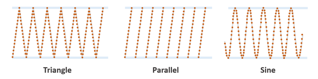
As a result, the same USGS document specifies to only use what they call the usable part (typically the center 95 percent) of a swath for evaluating the point density of a LiDAR data set.

Aggregating Point Clouds

One major advantage of LiDAR data compared to aerial photographs is that different datasets can be merged into a unified point cloud. By combining multiple layers of points, the point density within an area will increase accordingly. Such layers can come from multiple passes over the project area, flying with an overlap of over 50%, as well as from multiple channels or multiple sensors on a single collection platform.

Common Point Densities

Knowing about the nominal definition of point density, the obvious next question is: where do I need which point density? The point density requirement of a project will be a major factor contributing to the overall cost of a LiDAR project. While there might be various considerations for picking a certain point density, the level of detail that needs to be visible in the dataset will at least set the minimum point density. A higher point density will have a smaller point spacing and therefore reveal more features in the point cloud than sparse data.

Below are a few common point densities and how they are used. Bear in mind that technologies are evolving fast and even today a trend towards denser point clouds can be observed in many of these applications.

Sparse point clouds (0.5-1 pts/m²)

Point clouds with such low point densities are normally collected for large-scale digital height models. Subsets of these point clouds (either based on return number or classification) are used to create surface layers like the digital terrain model (DTM), digital surface model (DSM), normalized height model or the canopy height model used in forestry applications.

Low density point clouds (1-2 pts/m²)

At this point density, the point spacing is between 0.7 and 1 m. This can be enough for flood modeling applications, where even rivers and streams can be detected under forest canopies.

Medium density point clouds (2-5 pts/m²)

Very often a compromise between point density and cost of acquisition, these datasets are suitable for most uses. They might not be dense enough for 3D building modeling, but they can certainly be post-processed and analyzed to derive new products.

High density point clouds (5-10 pts/m²)

3D city modeling is one of the examples where a high point density will be required in order to capture the details of buildings. 5-10 pts/m² can be enough in order to capture the basic shapes of a building.

Extremely dense point clouds (10+ pts/m²)

Do you want a more detailed model of your buildings? In that case, you will certainly need a higher point density to capture all the details. For extremely high point densities, it might also be worth looking at other technologies, either instead of airborne LiDAR scanning or as an additional data source.