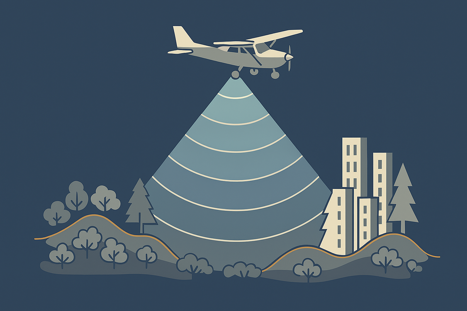
The fundamental basics of airborne LiDAR scanning are fairly simple. As explained in my introduction post about LiDAR technology, it is not much more than emitting a beam of light towards a target and measuring the time it takes to return to the sensor.
Looking a bit closer at this technology, though, we can see how the laws of physics start to introduce limitations on how LiDAR can be used. One of these limitations is a so-called “range gate” which I will try to explain in this post.
Introduction to range gate
The term “range gate” essentially describes the distances that can be measured by a certain LiDAR sensor. The minimum can be limited either by sensor specifications or for safety reasons (e.g., eye safety). On the far end, though, the range gate is restricted by the characteristics of the emitted signal. More precisely, it is the association of the emitted pulse with the returning pulse which becomes more challenging with higher pulse rates.
Calculating the maximum range of a single pulse
The emitted signal of a LiDAR sensor travels at the speed of light. As a result, the distance d between sensor and target can be calculated by d = c * t/2, where t represents the time between emitting the signal (E) and receiving the signal (R). The time is divided in half as the light has to travel the distance in both directions.
Applied to a timeline, this looks as follows:
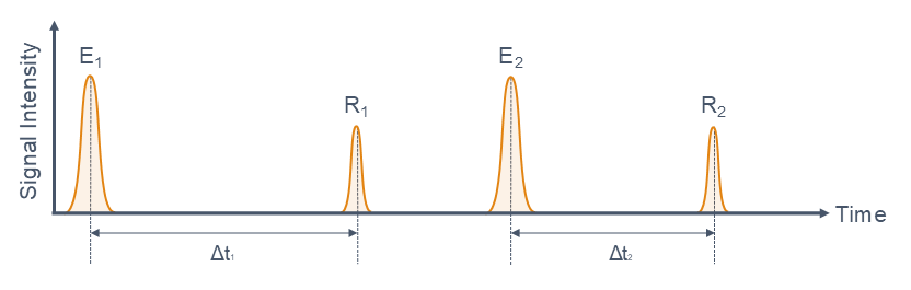
The limitation mentioned before arises when we have repeating pulses and we want to avoid ambiguities of the signals. In our timeline this means that the signal has to return to the sensor before the next signal is emitted. For a sensor with a given pulse-repetition-frequency (PRF) this time limit is t(limit) = 1 / PRF. Using the speed at which the light pulse travels (speed of light) the maximum distance the signal can travel is therefore: d(max) = c / PRF and the maximum distance between sensor and target: d(target) = 1/2 * c / PRF. This distance is called the maximum unambiguous measurement range.
(In reality, further factors, such as signal processing and internal electronics, will reduce the time limit even further. The resulting shortening of the measurement range can be as much as 400-500 m on older equipment. As this is highly system-specific, though, I am going to disregard it for the scope of this article.)
Second-time-around, third-time-around … multiple-time-around
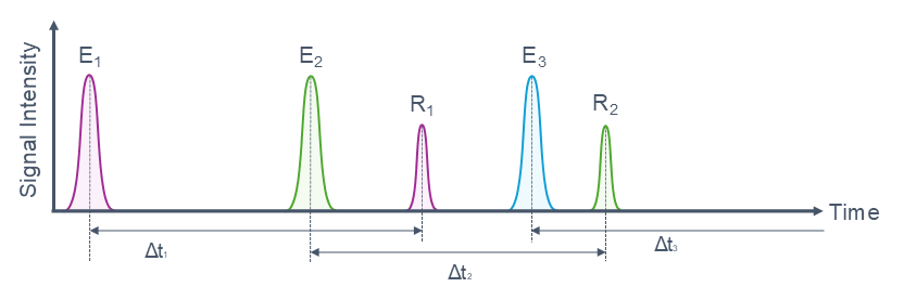
If the time of flight exceeds the pulse repetition interval, the emitted signal will get associated with the received signal from the previous emission.
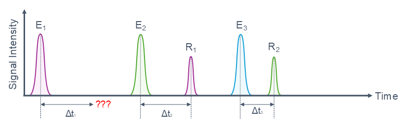
In order to get the correct range, the sensor would therefore have to wait for the second signal to be received. This signal which has a time delay exceeding one but not two pulse-repetition intervals is referred to as second-time-around echo. Correspondingly, echoes between two and three intervals are called third-time-around and so on. Together these echoes are sometimes called multiple-time-around echoes.
How to achieve high pulse densities from high altitudes
We are all looking for denser point clouds. The most obvious approach to achieve that is to send out LiDAR pulses more frequently. Unfortunately, as we can see from the formulas mentioned before, this will directly affect the maximum unambiguous measurement range.
Looking at the development of past years, it is fairly obvious that LiDAR sensor manufacturers have found ways to increase the collected pulse densities while coping with range ambiguities.
Sending coded LiDAR pulses
The problem of ambiguous return signals comes mainly from the fact that all signals are equal. Introducing an extra method (e.g., coding) of distinguishing between emitted signals makes it possible to have multiple pulses traveling in the air. By doing so, it is no longer the pulse repetition frequency but more the repetition frequency of a certain (coded) pulse type that limits the measurement range.
Having, for example, two different types of emitted signals would halve the pulse repetition frequency and therefore double the maximum unambiguous measurement range. The resulting formula can be described as d(max) = (m * c) / (2 *PRF), where m is the number of different signal types.
Splitting the emitted LiDAR signal
In recent years, manufacturers have started to use prisms to split the emitted laser beam into two individual signals. This way, the pulse repetition frequency can be maintained while doubling the number of returns collected.
However, splitting the laser beam also lowers the pulse’s power. For applications where successful collection of returns depends on the power of a LiDAR signal (e.g., forestry penetration), this methodology could potentially impact the quality of the resulting point cloud.
Adding additional signal emitters
Another way of increasing the pulse density without changing the pulse repetition frequency is duplicating the sensor electronics. Adding another emitting/receiving unit will also double the number of signals.
In order to further spatially decouple these multiple scanning components, they can be installed at an angle to each other. Additionally, these separate signals can have different wavelengths, which makes it possible to detect different features of the surveyed target.
Dealing with multiple-time-around echoes during post-processing
The problem of ambiguity comes from the fact that we are measuring an unknown distance. The measured object can therefore be at the distance retrieved from any of the multiple-time-around echoes. Introducing some restricting a priori knowledge to the survey project will eliminate many of these signals as a valid return. This can either be done by specifying in which time window the return signal is expected (MTA zone) or by supplying a rough surface model which can then be used to determine the echo to be used for processing.
Summary
There are many ways in which LiDAR sensor manufacturers handle the physical limitations of echo ambiguity. All have their advantages and disadvantages which I tried to summarize in the table below.
| Method | Advantages | Disadvantages |
|---|---|---|
| Coding pulses | Reduces the pulse repetition frequency and therefore increases the measurement range. | Decoding pulses needs extra processing. |
| Splitting signals | Doubles the number of pulses emitted while maintaining the pulse repetition frequency. | Emitted pulses have reduced power and might therefore result in weaker returns. |
| Adding additional signal emitters | Increased number of pulses (potentially even delivering additional attributes of the target). | More sensors result in higher hardware cost. Point pattern depends on configuration between emitters. Additional complexity. |
| Post processing | Tuning of parameters possible during processing | A priori knowledge of survey area (terrain) needed |