LiDAR Calibration and Strip Adjustment

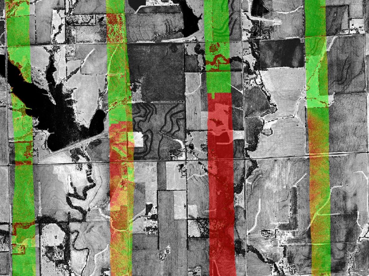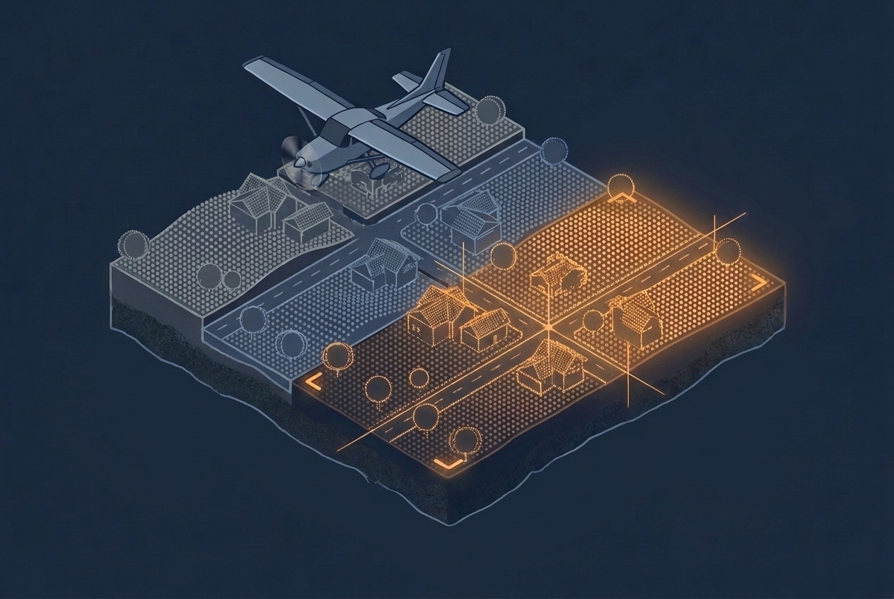
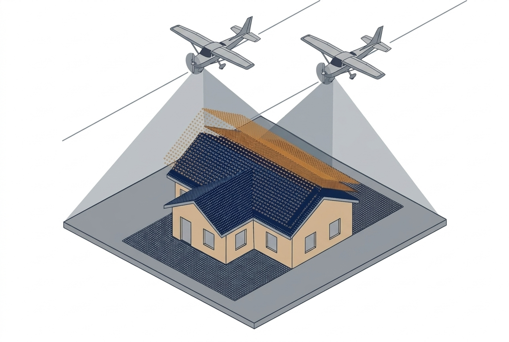
If you have worked with airborne LiDAR, you have seen it. You load two overlapping flightlines, and a roof appears twice, one point cloud sitting a few centimeters above the other. A road shows a small height offset exactly where one strip ends and the next begins. Perhaps you manually applied a shift, accepted the offset as it was, or sent the data back to the original provider asking them to fix it. So where do these differences come from, and what does it take to make the individual point clouds align with each other?

The answer lies in how LiDAR places its points. In photogrammetry, the shared camera position and orientation of each image helps provide rigidity across the observed scene. There is movement between individual images, but tie points across overlapping images help to connect the individual snapshots into a strongly connected block. LiDAR instead relies on direct georeferencing. Every point is positioned using the aircraft trajectory from GNSS and the IMU, combined with the angle and range of each laser pulse. Any small error or drift in measurement throughout that chain moves the point or even the whole strip. On its own, a single flight line is not rigid. But by bringing in other adjacent flight lines or control points we can achieve the same connectivity of a block that we know from photogrammetry.

In this article we look at the two approaches that are used to remove those errors: project calibration at the start of a project and strip adjustment during post-processing. We also cover the two common ways to align LiDAR data (surface matching and feature matching), and how images captured on the same flight or ground control points can help correct the point cloud.

Where the Mismatch Comes From

The errors come in two kinds. First are systematic errors as a result of how the system is built. The IMU and the laser scanner are mounted together, but never in perfect alignment. The small angular differences between them in roll, pitch, and heading are called boresight misalignment. Because this error is the same on every line, it leaves predictable patterns. A roll error tilts the strip, lifting one edge of the swath and lowering the other. A pitch error shifts the data along the flight direction, and a heading error mixes both. When two lines are flown in opposite directions, these errors point in opposite directions. The difference between the two strips is therefore twice the error, which makes the mismatch clearly visible where they overlap.

The second kind changes over time. The trajectory solution drifts as satellite geometry changes, as the aircraft moves away from the GNSS base station, and as the IMU accumulates small errors. These errors differ from one line to the next, and even more between flights on different days. No single correction removes them all.

Both kinds of errors affect two different properties of a dataset. Relative accuracy describes how well the strips agree with each other. Absolute accuracy describes how well the whole dataset agrees with the real world. Strips can match each other perfectly and still sit ten centimeters too high. Keep this distinction in mind, because it decides which step fixes which problem.

Project Calibration at the Start of a Project

Calibration happens in layers. The manufacturer already calibrates the sensor at the factory before delivery. That said, a boresight calibration is still needed every time the sensor is installed in an aircraft, since mounting changes the alignment. Many providers therefore fly a project calibration at the start of each project (or at least after the sensor has been freshly installed into an aircraft), to confirm the system behaves as expected and to solve the systematic angles with data from that exact installation.

A calibration flight follows a specific pattern over a carefully selected site that contains both flat and sloped surfaces, ideally buildings with roofs facing different directions. The exact pattern varies between providers, but it usually combines lines flown in opposite directions, lines that cross each other, and more than one altitude. A common design flies two opposing lines at one altitude and two crossing lines at roughly double that height. Each of these elements matters because each error only reveals itself under a specific geometry. Opposite lines expose roll and pitch errors, while crossing lines and a change in altitude help separate heading errors from the rest.

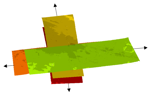
Doing this at the beginning of a project makes it possible to find systematic errors once, so that the corrections can be applied to the sensor calibration before collecting any additional data. Unusually high errors can also indicate that the hardware itself has a problem, and that it might be good to investigate these issues before spending time and money collecting project data that might be of little use in the end.

Matching During Post-Processing

Once the calibration values are applied, the remaining errors are mostly the ones that change over time. Strip adjustment, often simply called matching, compares every pair of overlapping strips and computes small corrections so that they fit together. It usually works in stages: first a correction per flight to remove offsets between days, then a correction per line, and sometimes a correction that varies along a single line.

This is also one of the real reasons flight plans include overlap between lines. The more overlap, the more shared ground the algorithm can use to compare flight lines. At the same time, higher overlap means less efficiency in covering the project area. In the end, it is a trade-off, set either by the project specifications or by the flying company based on experience.

Project calibration and matching during post-processing rely on essentially the same methods, described in the sections below. The difference lies in the data used for matching. Calibration works on a dataset collected specifically for that purpose, with a flight pattern designed to expose each systematic error. Matching works on the project data as it was flown, with whatever geometry the project provides.

But how does the algorithm compare data from two flight lines? Laser points never land on exactly the same spot twice, so algorithms have to find other ways to compare the point clouds. There are two approaches that are commonly used that we will look at in the sections below.

Surface Matching

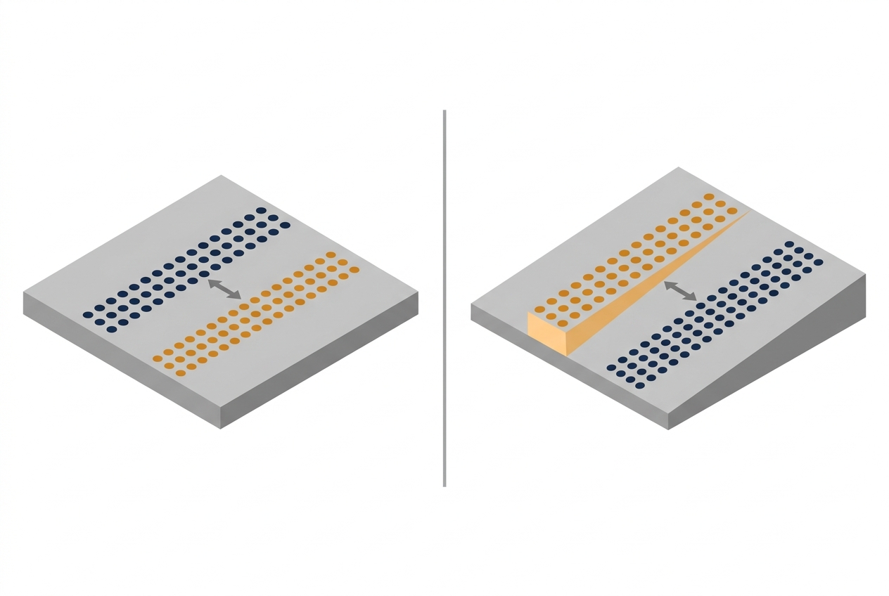
Surface matching treats each flight line as one continuous surface. It compares the full overlap between two strips and moves and/or rotates data of one strip until the two surfaces fit as closely as possible across the whole shared area. Nothing needs to be picked out in advance, since every relevant point in the overlap contributes to the result.

This works as long as the surfaces vary. A flat surface only reveals a vertical offset. Slide a strip sideways over a flat parking lot and nothing changes, so a horizontal error stays invisible. A slope turns a horizontal shift into a height difference, and that is what the method can measure. Surface matching therefore works best in open, varied terrain and struggles in flat areas with few distinct shapes.

Feature Matching

Feature matching aims to lighten the workload of the adjustment. Instead of comparing whole surfaces, it picks out distinct elements that appear in strips and matches only those. The features can be lines, such as roof ridges, building edges, or break lines on slopes, or patches, such as roof faces and small sections of sloped ground. Each feature is defined by many points, which makes it far more precise than any single point on its own. When the features are lines, the approach is often called tie line matching.

Features pin down horizontal position well, especially when they run in many directions. They can also be tied to positions measured on the ground, which links the relative matching of strips to absolute accuracy. The weakness is that the method depends on finding enough distinct features, facing in enough different directions. In rural or forested projects, few usable features exist, and too few tie features lead to unreliable corrections.

Correcting the Trajectory or Bending the Points

Whichever method finds the corrections, applications differ in how they apply them. Some do not apply them to the point cloud directly. Instead, they tie them back to the trajectory. Rather than shifting or rotating the points, they adjust the position and orientation of the aircraft along its flight path and then recompute the points from the corrected trajectory. Every point is still derived by following the measurements of the sensor, whereas the updated flight path keeps the whole strip together.

The trajectory corrections also hint at where the errors came from. A consistent residual error across multiple flights can indicate problems with the calibration. If the errors are limited to one flight line, or part of one, they more likely come from local drift, a short GNSS outage, or a change in satellite constellation.

Other algorithms go one step further, and this is where things get complicated. Instead of correcting the trajectory, they bend individual areas of the point cloud into agreement, much like rubber sheeting known from the GIS world. This helps to eliminate even the smallest remaining differences that cannot be explained by errors of the sensor model, but the price is that the adjusted points no longer follow the model of how they were surveyed, essentially breaking the connection between point and trajectory.

Does this disconnect matter? It does for any processing step that uses the trajectory again. Many software packages ask for both the point cloud and the trajectory, because they reestablish the connection between the two and use it during processing. That only makes sense if the link was not broken during the alignment step. If points were adjusted freely, the resulting sensor-to-point path is shifted as well. Any assumption that is based on this path (like for example that there are no objects along this path) could potentially be incorrect and affect further processing results.

Classify Before You Match

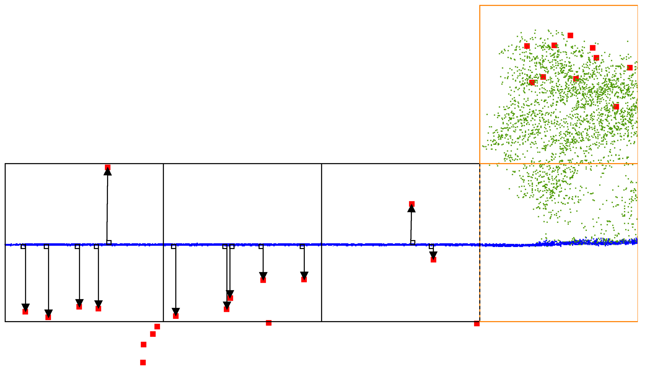
Both methods work best on a classified point cloud. A raw strip contains everything the laser hit: treetops, cars, people, birds, and stray noise points above and below the ground. Many of these are not the same in two passes. Leaves move in the wind, a car drives out of the scene, and a noise point exists in one strip only. If matching considers all of them, it tries to fit strips to things that were never stable, and the corrections suffer.

Classifying first, usually separately for each flight line, lets matching use only points whose meaning is known. Ground and roof points become the surfaces and features that matching relies on, while vegetation and noise stay out of the calculation. The classification does not need to be final at this stage. It only needs to be good enough to separate stable surfaces from everything else.

Choosing Between Them

The terrain usually decides. Urban areas with many buildings favor feature matching. Open, hilly terrain favors surface matching. Forest and flat farmland are the hardest cases, where processors rely on ground points under the canopy and whatever slopes and structures exist, often combining both methods. Most processing tools support both approaches for this reason.

Matching is designed for the small errors that remain after calibration. If a large systematic error was never calibrated out, matching may reduce the visible seams without fully removing the cause. This is why calibration at the start and matching at the end are complementary steps, not alternatives.

Using Other Data Sources to Adjust the Point Cloud

Sometimes the LiDAR strips are not the only information available. Many airborne systems carry a camera next to the scanner, and both sensors share the same GNSS and IMU trajectory. The images go through aerial triangulation, which uses tie points between overlapping photos to refine the position and orientation of every exposure. Those refinements are, in effect, corrections to the shared trajectory. Transferred to the LiDAR, they correct the point cloud as well, and the result is an optimized point cloud that fits the imagery.

This helps most where LiDAR matching alone is weak. Images often offer many distinct tie points in areas where the terrain is flat or has few structures, while LiDAR provides reliable heights where image texture is poor. The most rigorous version, called hybrid adjustment, solves the image block and the LiDAR strips together in a single adjustment instead of correcting one and passing the result to the other. It works best when camera and scanner fly on the same platform, because the shared trajectory is what connects the two datasets. The same idea applies to other reference data of known quality, such as control surfaces measured on the ground.

A side benefit is consistency between products. When LiDAR and images are adjusted separately, the point cloud and the orthophoto can disagree by a noticeable amount. Adjusting them together, or transferring corrections from one to the other, keeps both products in the same place, which matters as soon as someone colorizes the point cloud or overlays the two in a map.

What This Means When You Evaluate a Dataset

You rarely see these steps, but you can ask about them. Was a calibration flight flown for this project, and over what kind of site? Was the point cloud classified before matching, and which matching approach was used for the terrain? If images were captured on the same flight, were they used to support the adjustment? How large are the remaining differences between overlapping strips, and how were they measured? And was absolute accuracy checked against independent ground control, separately from how well the strips match each other? National specifications such as the USGS Lidar Base Specification set limits for differences between overlapping swaths, which gives you a reference point for the answers.