Pulse Repetition Frequency

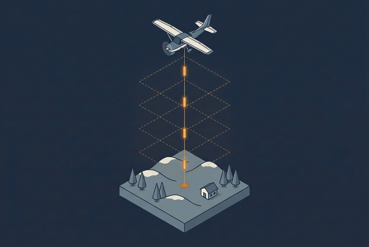
Open the specification sheet of a current airborne laser scanner, and the pulse rate is usually the headline number. Two million pulses per second on a single channel is no longer unusual. Read a little further down the same sheet, though, and a second number tells a quieter story. One dual-channel sensor can operate at up to about 3,900 meters above ground at its lowest pulse rate, but only up to about 1,700 meters at its highest. The faster the scanner fires, the shorter its reach. So why does firing more often cost range, and how do modern sensors fire more often than the speed of light used to allow?

Pulse repetition frequency appears in almost every article on this blog. It controls the spacing of points across the swath when you change the aircraft speed, it works together with the scan pattern to distribute points on the ground, and it is the main reason one survey delivers two points per square meter while another delivers twenty. In this article we define what PRF actually measures, look at why raising it reduces the energy in every pulse, explain how the travel time of light puts an upper limit on the rate, and show how multiple pulses in the air works around that limit. Together, these explain why PRF is the setting that most directly connects the cost of a survey to the density of its data.

What Pulse Repetition Frequency Measures

Pulse repetition frequency, or PRF, is the number of laser pulses a scanner emits per second. It is given in kilohertz, so a sensor set to 400 kHz fires 400,000 pulses every second. Some manufacturers call it pulse repetition rate (PRR). Both terms describe the same thing.

Not every emitted pulse becomes a measurement on the ground. Scanners with a rotating polygon mirror, one of the designs covered in the scan pattern article, spend part of each rotation pointing away from the ground. NEON, which operates several airborne LiDAR systems for ecological monitoring in the United States, notes that only about two thirds of the pulses of its rotating-mirror sensors are fired toward the ground. A setting of 400 kHz therefore delivers about 266 kHz of usable measurements. For this reason, specification sheets often list both a pulse rate and an effective measurement rate, and only the second one reaches the ground. In the other direction, a single pulse can produce several returns in vegetation, so a point cloud can contain more points than pulses. This is why the USGS counts only last returns when it checks point density.

With those details in place, the link between PRF and density is simple. Divide the effective measurement rate by the area the aircraft covers every second, which is its ground speed multiplied by the swath width, and you get the average number of pulses per square meter from a single pass:

Here v is the ground speed and w is the swath width. An example shows the scale. At 1,000 meters above ground with a 40 degree field of view, the swath is about 730 meters wide. Flying at 60 meters per second (about 117 knots), the aircraft covers roughly 44,000 square meters every second. With an effective rate of 400 kHz, that gives about 9 pulses per square meter. Double the rate and the density doubles. Alternatively, you can keep the density and fly twice as fast, or fly higher to cover a wider swath. That last option is where the physics starts to push back.

Why Each Pulse Gets Weaker as the Rate Goes Up

A laser source delivers a roughly fixed amount of average power. The energy of each pulse is that power divided by the number of pulses, so doubling the PRF roughly halves the energy in every pulse. A weaker pulse produces a weaker echo, and the echo has to stay clearly above the noise level of the receiver to be recorded as a return.

Because the returning signal fades quickly with distance, less energy per pulse means a shorter maximum range. This is the pattern behind the numbers in the opening. At its highest combined rate of 4 MHz, the sensor is specified to reach targets with 20 percent reflectance from about 1,700 meters above ground. At 540 kHz, the same sensor reaches about 3,900 meters. Reflectance matters as much as the rate. Dark asphalt, dark roofing, and wet surfaces reflect only a small part of each pulse, so they are the first targets to drop out when a sensor operates close to its range limit.

Pulse energy also affects what reaches the ground under a canopy. A pulse that passes through gaps in the foliage loses part of its energy at every leaf and branch it touches, and a weaker pulse has less left over for the ground. Lee and Wang studied this in a tropical forest and found that both a lower flying height and a lower PRF increased the share of pulses that reached the ground. Flying height had the much larger effect, though. Flying one kilometer lower raised the penetration rate by about 10 percent, while lowering the PRF by 50 kHz (and by doing so increasing the energy per pulse) raised it by about 2 percent.

Earlier research also found a small effect on range accuracy. Csanyi and Toth at The Ohio State University compared strips flown with the same sensor at 33, 50, and 70 kHz and found that the mean elevation error grew with the pulse rate, from about 4 to about 14 centimeters. A transformation of each strip, similar to the strip adjustment done in post-processing, removed those offsets. Sensor technology has moved on considerably since that 2006 study, but the principle remains: less energy per pulse leaves less margin.

How the Speed of Light Limits the Pulse Rate

Energy is one limit on the pulse rate. The other comes from how long each pulse needs to travel. A LiDAR sensor measures distance by timing how long a pulse takes to reach the ground and return. Light is fast, but not infinitely fast. From 1,000 meters above ground, the round trip takes about 6.7 microseconds. If the sensor waits for each echo before it fires the next pulse, it can fire at most about 150,000 times per second at that height.

For a long time, this is exactly how airborne scanners worked. Only one pulse was allowed in the air at any moment, so the maximum PRF was tied directly to the flying height. The distance at which this limit applies is called the unambiguous range, and it equals the speed of light divided by twice the PRF. At 100 kHz, the unambiguous range is 1,500 meters. At 1 MHz, it is only 150 meters, which is lower than almost any crewed survey flight.

What happens if the sensor fires anyway? The receiver still sees an echo, but it can no longer tell which pulse the echo belongs to. At 1 MHz, an echo that arrives half a microsecond after the latest pulse could come from that pulse hitting a target 75 meters away, from the pulse before it hitting a target 225 meters away, or from the one before that at 375 meters. This is called range ambiguity. For sensors that could handle only one pulse at a time, the only answer was to keep the PRF low enough that it could not happen. It is also why the aircraft speed article recommends a lower PRF when a strip contains large differences in elevation.

Firing the Laser With Multiple Pulses in the Air

In the mid-2000s, manufacturers started to break the link between pulse rate and flying height. The idea behind multiple pulses in the air (MPiA), which RIEGL calls multiple time around (MTA), is to fire the next pulse before the previous echo has returned, and to work out afterwards which pulse each echo belongs to. The space below the aircraft is divided into zones that are each one unambiguous range deep. Zone one contains targets closer than one unambiguous range, zone two contains targets between one and two, and so on. As long as the sensor or the processing software knows which zone the ground is in, every echo can be assigned to the pulse that produced it.

The effect on productivity was immediate. Roth and Thompson described an early large-area project in which two pulses in the air made it possible to reach the required density at twice the coverage rate, or twice the density at the same coverage rate. Current high-end sensors go much further. The dual-channel sensor from the opening is specified to handle up to 45 pulses in the air at the same time.

Assigning echoes to zones is the difficult part. The sensor needs to know roughly how far away the ground is, and that distance changes with terrain, buildings, and the altitude of the aircraft. Where the ground crosses from one zone into the next within a strip, echoes are harder to assign, and two kinds of problems can appear. Echoes that arrive at the same moment the sensor fires its next pulse can be lost, which leaves gaps in the data. Echoes assigned to the wrong zone produce points that are displaced by a whole unambiguous range, so they show up as scattered noise far above or below the actual surface.

Manufacturers solve this in different ways. Some vary the timing between pulses slightly, so that echoes assigned to the wrong zone do not line up into a surface and are easy to filter out. Others resolve the zones during processing by checking each result against the expected terrain, as in the gateless MPiA approach Leica Geosystems presented for sensors operating across very different altitudes and terrain. Terrain relief still matters for flight planning, however. In steep terrain or over tall buildings, the ground below a single strip can span several zones, and planners take this into account when they choose the pulse rate and flying height for each part of a project.

Choosing a Pulse Repetition Frequency for a Project

With pulse energy and range ambiguity in mind, PRF becomes a setting with a clear trade-off. A higher rate delivers more pulses per second, which the flight plan can spend on density, on speed, or on a wider swath from a greater height. A lower rate delivers stronger pulses that reach further, return reliably from dark surfaces, and have a better chance of reaching the ground below dense canopy. MPiA removed the hard limit that the speed of light placed on the rate, but it did not remove the energy trade-off.

Which way a project leans depends on its purpose. A national terrain program with a modest density target benefits from flying high with a wide swath, which pushes toward lower rates to keep enough energy in each pulse. A city model or a utility corridor with a high density target is flown lower, where the full rate is available and each pulse still has enough energy. Forest projects, such as the repeat surveys used to track forest growth, need enough ground returns under the canopy, so the gain in penetration from flying lower is often worth more than the time saved by a higher rate. Multi-channel sensors add one more option. Two lasers sharing one scanner double the total pulse rate without dividing the energy of a single laser between twice as many pulses, which is how the highest current rates are reached.

In practice, survey companies rarely look for a single ideal rate. They choose the highest rate that still returns reliable echoes from the darkest and most distant targets in the project area. Every additional pulse per second translates into flying time saved, and flying time is one of the largest factors in the efficiency of an aerial survey.

What to Ask When You Evaluate a Dataset

PRF rarely appears in a delivery report on its own, but you can ask about it. Which PRF was used, and is the quoted number the pulse rate or the effective measurement rate? How does the flying height compare with the maximum range the manufacturer specifies for that rate on low reflectance targets? In forested areas, how many last returns reached the ground below the canopy? And for sensors operating with multiple pulses in the air, how were zone assignments checked, and how were the resulting noise points classified? A provider who planned the survey carefully will have these answers ready.

PRF only describes how often the sensor fires. Where those pulses land across the swath depends on the field of view and the scan pattern, and how they add up across neighboring strips depends on the overlap between flight lines. All of these settings share the same budget of pulses, and seeing them together is what turns a specification sheet into a flight plan.