Watching Point Clouds Grow

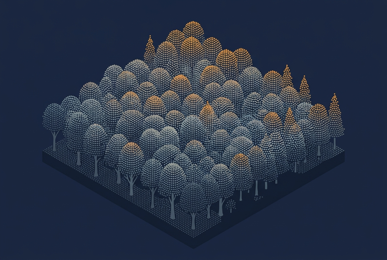
Every year, aerial survey contractors fly LiDAR sensors over three and a half to four million hectares, part of a six-year cycle that eventually covers every corner of the country. That is a lot of area to scan. When I mention this to friends and colleagues, they often wonder what could possibly make it worth flying over all these areas that are essentially just trees.

The interesting part is what happens after the flight lands. The Finnish Forest Centre turns those points into a forest resource database that foresters, timber buyers, and land managers actually use. For each stand, it holds standing volume per hectare, growth rate, and harvest readiness, and the whole database gets updated on a regular schedule.

You already know how a LiDAR point cloud gets built from scan pattern and pulse density. Turning that cloud into actionable insights, such as tons of biomass per hectare or a growth rate over time, requires a separate process.

Let’s look at how canopy height, crown structure, and wood volume derived from a point cloud turn into a biomass estimate. Forestry inventory is the main example we will follow, with wildfire fuel load and utility corridor vegetation management coming in as applied cases along the way. After reading it, you will understand why flying the same ground twice gives you more than two separate measurements. Match the same trees between flights, and you can read off exactly how much each one gained or lost, rather than estimating it from a model.

From Canopy Height to a Biomass Number

A LiDAR point cloud over a forest already contains the pieces needed for a biomass estimate: a digital terrain model showing bare ground (DTM), a digital surface model showing the top of the vegetation (DSM), and the difference between the two, the canopy height model (CHM), showing how tall the vegetation is at every point in the area. None of that is new if you have followed the earlier articles in this series.

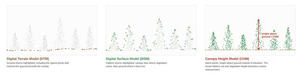
This next step is often skipped in introductions to LiDAR forestry: a canopy height model is height, not biomass. Getting from one to the other takes an allometric equation, a formula built on the fact that as a tree grows, its different measurements grow together in predictable ways.

Foresters have used allometric equations for decades. They measure a tree by hand using a tape around the trunk for diameter and a clinometer for height. Combined with a wood density value taken from published tables for that species, these measurements give an estimate of stem volume or dry biomass.

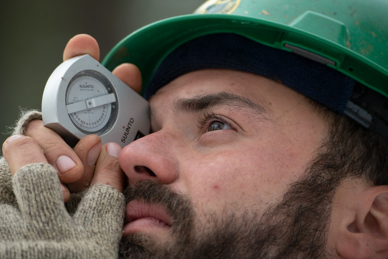
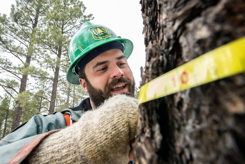
Airborne LiDAR does not replace that logic. It replaces the tape measure. Instead of diameter at breast height, the equation uses height statistics calculated from the point cloud within a plot, such as the mean height of the tallest returns, height percentiles, the standard deviation of heights, and the percentage of the plot covered by canopy. These plot-level numbers are used instead of measuring each tree by hand, since individual trees are usually not visible from the air under a closed canopy, which is most of the time.

Why the Same Equation Will Not Work in Every Forest

The trouble with allometric equations is that they are fitted to a specific set of trees, not derived from a formula that works everywhere. A calibration only holds where it was built. A model trained on Norway spruce in Switzerland does not automatically apply to Scots pine in Finland, and often not even to a Scots pine stand two hundred kilometers away with different soil and stocking density.

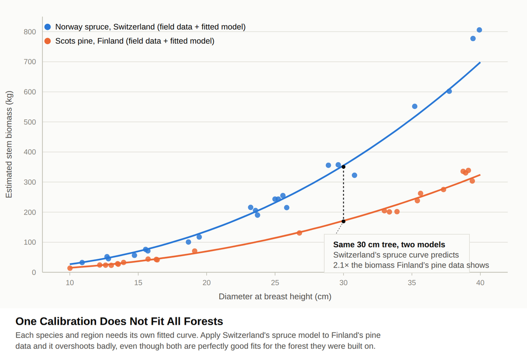
The published wood density values used in the equation have their own uncertainty. This comes from differences in how the wood was measured, where the sample trees grew, and how many trees were sampled. That uncertainty can be as large as the effect the model is trying to measure. Diameter at breast height also becomes a weaker stand-in for tree size as canopy shape becomes less regular. In mixed-age or multi-layered stands, the simple chain of assumptions, that height predicts diameter, and diameter predicts volume, starts to break down.

This is why every serious biomass mapping program pairs its LiDAR data with field plots. It is also why the Finnish Forest Centre’s flight cycle is only part of the process. Each inventory area is matched with 700 to 800 circular sample plots, or 150 to 200 of a newer, larger tree-map plot design. These plots are measured on the ground and used to calibrate the model before it is applied to the rest of the LiDAR coverage. The plots are not just a routine step. They are what allows a national program to say its LiDAR-derived numbers are accurate for that particular part of the forest.

Applying that calibration to an entire country raises a further question: use one national equation, or let the data itself define which plots and stands are most alike. Sweden’s national forest attribute map, built from airborne laser scanning combined with National Forest Inventory field data, used the second approach. It works by looking at each unsampled area of forest and borrowing the values from the field plots whose LiDAR data looks the most similar, instead of running everything through one fixed formula. Statisticians call this method k-nearest neighbor.

A recent review published in the journal Forests looked across many published studies on LiDAR-based biomass estimation and found that about two-thirds of those studies still use standard regression, a formula fitted once and then applied everywhere. About one in five of the same studies use more flexible, data-driven approaches instead, including one statistical technique that is confusingly called random forest (it actually has nothing to do with forests), and the rest combine both. These flexible approaches are becoming more common because they can handle regional differences and complex patterns better than one fixed formula can.

What a Second Flight Buys You

A single LiDAR acquisition gives you a snapshot, biomass or volume as it stood on the day the aircraft flew. Collecting the same data over the same ground at a different time gives you a second snapshot, and lets you measure the change between the two, in much more detail than most people expect.

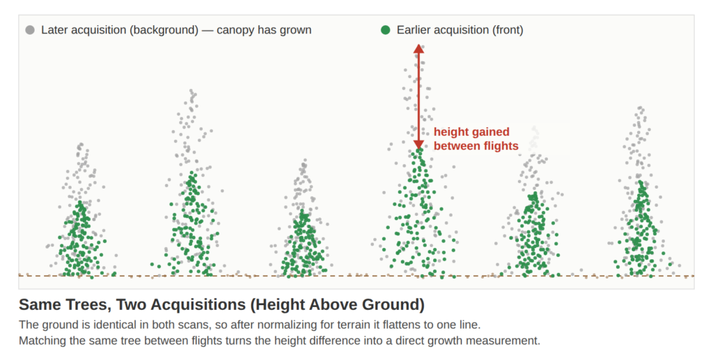
Instead of estimating growth with a generic formula for the species and site class, researchers can measure it directly, an approach demonstrated in a study published in Ecology and Evolution. They identify individual tree crowns in each acquisition and match the same tree between the two flights, using its position and crown shape. Then they measure exactly how much height or crown volume that tree gained, or lost if it died or was harvested. This is a different kind of number than a model’s growth prediction: it comes from measuring the same tree twice.

I worked on a smaller-scale version of that crown-modeling problem years ago. We fitted mathematical models of individual tree crown shapes to LiDAR points, across more than 15,000 reference trees in Hyytiälä, Finland. That project had a different goal of classifying tree species from calibrated aerial imagery, not estimating biomass. Still, the crown models were accurate to within about 35 centimeters of radius, compared to field measurements. That shows how well a point cloud can support a fitted shape, once you treat it as a surface to be modeled rather than just reading the highest point in each pixel.

Other Uses for the Same Point Cloud

Not everyone who uses a point cloud wants a biomass number, though. Two other applications start from the same LiDAR-derived canopy structure and lead to a completely different result.

Wildfire management cares less about total standing biomass than about which fraction of it can actually catch fire. Canopy bulk density and crown fuel base height are the inputs that fire behavior models such as FARSITE and FlamMap need, as detailed in a paper published in the journal Fire. These describe the density of burnable live and dead material within the canopy and the height to the bottom of that live fuel, not the amount of wood stored in a trunk that will not easily ignite. LiDAR-derived vertical profiles, height percentiles and canopy returns grouped by height, feed the same kind of flexible, data-driven models discussed above, but what is being measured has shifted from mass to flammability. A stand with high biomass and a high, clean crown base can carry much less fire risk than a lower-biomass stand where fuel runs continuously from the ground into the canopy.

Utility corridor vegetation management asks a simpler question of the same point cloud: is any vegetation too close to a conductor. Here the workflow skips allometry entirely. As Microdrones describes, once a classification step separates vegetation points from the classified power line and tower points, software such as LP360 draws concentric clearance buffers around each conductor, at distances such as 10, 7.5, 5, and 3 meters, and flags any vegetation return that falls inside them. A drone-mounted LiDAR sensor can survey a kilometer of corridor in roughly ten minutes at that resolution. No biomass model is involved because none is needed. Encroachment is a geometry problem, not a mass problem, and the point cloud answers it directly.

That contrast is the main point. The same raw point cloud can support a mass-and-volume model when the decision concerns carbon accounting or timber value, or a distance-and-threshold check when the decision concerns asset risk. Neither approach is more correct than the other, they are simply built for different questions. What connects them is the value of doing it twice. A biomass estimate calibrated against field plots tells you what a forest is worth today. A repeated acquisition, whether that is Finland’s six-year national cycle or a utility’s annual corridor survey, tells you whether that value is growing, shrinking, or slowly becoming a hazard. That difference, between a single measurement and a trend, is where most of the practical value in forest LiDAR actually comes from.