How Temporal Resolution Shapes Geospatial Data

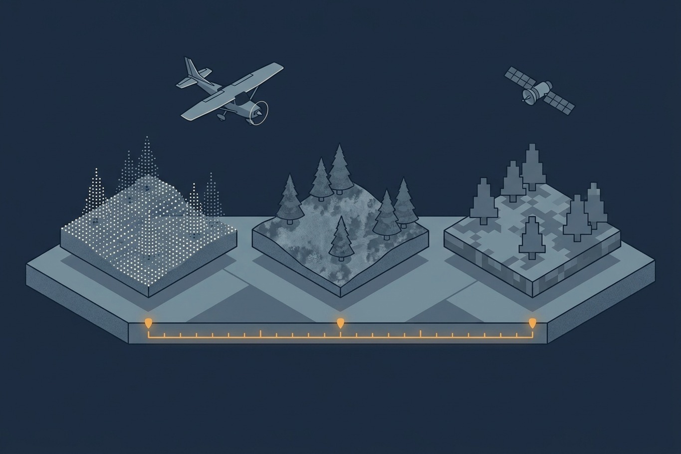
Open the forest map service of the Swedish Forest Agency, and you will find two tree height layers for the same forest. One is called tree height from laser, the other tree height from aerial images. Zoom into a young stand, and the two can disagree noticeably. Neither layer is wrong. They were simply captured in different years, and the trees kept growing in between. The same agency also warns that stands harvested during the winter will not disappear from its maps until spring. Which layer should you trust, and why does a national program deliberately keep several versions of the same forest?

The answer lies in temporal resolution, the dimension of a dataset that is easiest to overlook when you evaluate it. We usually judge geospatial data by how much detail it contains: the point density of a LiDAR survey, the pixel size of an image. How often that detail is renewed gets far less attention, even though it decides whether a dataset still describes the world you are making decisions about. In this article we define temporal resolution, look at why it trades off against spatial detail, and use Sweden’s national elevation and forest mapping program as an example of how three different update cycles can be combined. We end with a simple way to judge whether the timing of a dataset fits the question you want to answer.

What Temporal Resolution Means

Temporal resolution describes how often the same place is observed. For a satellite, it is the revisit time, the interval between two passes over the same location. For an airborne program, it is the repeat cycle, the number of years until the same area is flown again. A weather satellite in geostationary orbit may observe the same area every few minutes, while a national LiDAR program might return only every five to ten years.

The revisit time is not the same as the number of useful observations, though. An optical satellite that passes every few days sees nothing through clouds, and at northern latitudes it sees very little during the dark winter months. Airborne programs have their own version of this. A country is never flown in a single day. It is captured block by block over several seasons or years, so a national dataset is really a mosaic of acquisition dates. Two neighboring tiles can be several years apart, even though they carry the same product name.

This leads to a second number that matters more in practice: the age of the data at the moment you use it. A program with an eight-year cycle delivers data that is anywhere between a few months and eight years old, depending on where you look and when. Temporal resolution tells you how often the data is renewed. The age of the data tells you how far it may have drifted from reality since the last update.

Two more details decide what a date actually tells you. The first is the season. A survey flown in spring, before the leaves come out, shows more of the ground. A summer survey shows the full canopy, and snow cover changes the surface altogether. Lantmäteriet, for example, captures its aerial images between mid-April and September. It tries to photograph southern Sweden before the trees are in leaf, then moves north as the snow melts. Two datasets from the same year can therefore describe quite different landscapes. The second detail is delivery time, the delay between acquisition and the moment the data becomes available. For a national LiDAR or image program, processing and quality control often take months. At the other extreme, NASA’s FIRMS service publishes satellite fire detections within about three hours. The age of the data at the moment you use it always includes this delay.

Why Detail and Frequency Pull in Opposite Directions

If frequent updates are so valuable, why not capture everything often? Because each acquisition has a cost, and that cost grows with the level of detail. A LiDAR flight that delivers several points per square meter over a whole country takes years of flying time, as described in the article on survey efficiency. Repeating it every year would multiply that effort. Satellites sit at the other end of the scale. They revisit every few days at almost no additional cost per image, but their pixels are measured in meters rather than centimeters, and an optical sensor can only see the top of the canopy.

Every data source therefore sits somewhere along the same trade-off between detail and frequency, and no single source covers both ends. New technology keeps shifting the balance. Commercial satellite constellations now deliver images with pixels below one meter of the same place almost every day, and drones can fly centimeter-level surveys whenever they are needed. The basic constraint remains, though: detailed data needs sensors close to the ground, and sensors close to the ground cover less area per hour. A drone can cover a construction site in a day, but a whole country would take years. A satellite image, however sharp, still shows only the top of the canopy. The practical question therefore becomes how to combine sources that each cover one end of the trade-off. Sweden offers a good example of how this can be done at national scale.

How Sweden Combines Three Update Cycles

Sweden’s national program is run jointly by the Swedish Forest Agency, the national mapping agency Lantmäteriet, and the Swedish University of Agricultural Sciences. It is built on three data sources, each with its own cycle.

The foundation is airborne laser scanning. The first national scan ran from 2009 to 2017, and the second, flown for forestry at roughly 1 to 2 points per square meter, ran from 2018 to 2025. A third cycle has already started in parts of the south and north. For any given area, that gives a repeat interval of roughly eight to nine years. From each scan, the agencies derive a ground elevation model and a set of forest attribute maps (tree height, stem volume, basal area, and biomass), calibrated with field plots from the National Forest Inventory. The attribute maps come with an explicit warning: they show the forest as it was in the year the area was scanned.

The second source is aerial imagery from the national image program. Lantmäteriet derives a surface model from aerial images by image matching, the photogrammetric technique that finds the same point in overlapping images and computes its height. New imagery covers about one third of the country each year, so the surface model is renewed roughly every three years. This is where the second tree height layer from the opening comes from.

The third source is satellite imagery. The Forest Agency uses satellite change analysis to detect clear-cuts and remove them from its maps long before the next laser scan. This is the fastest cycle, but it also has the clearest gaps: harvests carried out in winter only appear in spring, when usable images are available again. Storm damage is another weak spot, since the automated analysis can mistake wind-thrown forest for a harvested stand.

What makes the combination work is that the three sources are not interchangeable. Image matching only sees the top of the canopy, because the ground below a closed forest is hidden in every image. On its own, it would give surface heights above sea level, not tree heights. The laser-derived ground model supplies the missing piece. Subtract the ground from the image-based surface, and you get a current canopy height model. Bohlin and colleagues showed that this approach, combined with the same National Forest Inventory plots, maps tree height, volume, and basal area across central and southern Sweden with accuracy close to that of laser scanning. The laser data remains slightly more accurate, because it also records structure inside the canopy, but the image-based maps are renewed almost three times as often.

Why the Ground and the Canopy Need Different Cycles

The Swedish design rests on a simple observation: different parts of the landscape change at very different rates. The shape of the ground changes so slowly that a terrain model that is eight or nine years old is still an accurate reference almost everywhere. A forest canopy grows every season, and a harvest can remove it in a few days. Bohlin and colleagues note that forestry operations alone change about 3.5 percent of Swedish forest land every year. Over one laser cycle, that adds up to as much as a third of the forest. Each layer is updated at a rate that roughly matches how fast it changes.

The assumption has limits, and they are worth knowing. Where the ground does change, for example in a gravel pit, on a construction site, or along an eroding riverbank, an outdated terrain model is subtracted from a current surface, and the resulting canopy heights are wrong by exactly the amount the ground has changed. Young forests are a second weak spot. They grow fastest, so their laser-derived attributes age the quickest, which is where the two tree height layers from the opening are most likely to disagree. And any layer that is updated by automated change detection inherits the blind spots of its source, as the winter gap and the storm damage false positives show.

What It Takes to Compare Two Surveys

The same logic applies to repeated LiDAR flights over the same area. As described in Watching Point Clouds Grow, a second acquisition turns two snapshots into a measured rate of change, and temporal resolution decides how finely that rate can be resolved. Before any change can be measured, though, the two surveys have to be comparable. A difference between two surveys carries the error of both, so studies of repeat surveys use a level of detection, a threshold below which a difference cannot be separated from noise. With a vertical error of about 5 cm in each survey, that threshold lies at roughly 14 cm. A harvested stand stands out clearly, while a riverbank that dropped by a few centimeters stays invisible. Systematic errors are harder to catch. If one survey sits a few centimeters too high across a whole block because the trajectory solution drifted, every difference in that block shifts by the same amount. This is why repeat surveys are usually aligned on stable surfaces such as roads and roofs before they are compared.

The two surveys also rarely share the same specification. According to Skogforsk, Sweden’s first national scan captured about 0.5 points per square meter and the second at least 1. A sparse survey is more likely to miss the top of a tree, so part of the growth measured between the two scans can come from the denser sampling rather than from the trees. This gives the first survey of a program a role beyond its own use. It becomes the baseline that every later survey is measured against, and its specification limits which changes can ever be detected.

Matching Temporal Resolution to the Question

The Swedish example points to a framework you can apply to any dataset. Start with the thing you want to measure and ask how fast it changes. Then compare that rate with two numbers from the dataset: how often it is renewed, and how old it is in the place and at the moment you need it. If the phenomenon changes faster than the data is renewed, the dataset can describe a state, but it cannot follow a process.

Wildfire management shows how wide the range of required cycles can be within a single application. In his overview of remote sensing for wildfires, Georgios Zagalikis describes how the data needs shift from before a fire to during and after it. Sorted by how quickly each factor changes, they span everything from decades to hours. Fuel structure, such as the canopy bulk density derived from LiDAR, fits a multi-year airborne cycle, while an active fire is followed by satellites that pass over several times a day, even though their pixels are coarse.

No single dataset covers all of these time scales, and none needs to. The skill lies in recognizing which time scale each part of a question belongs to, and in choosing a source whose cycle is at least as fast as the change it has to capture. Sometimes that points to an expensive new acquisition. Just as often, it shows that an older, detailed dataset is perfectly adequate for the slow-changing part of the problem, and that a cheaper, more frequent source can cover the rest.

What to Ask When You Evaluate a Dataset

The date of a dataset is rarely printed on the map, but you can ask about it. When was the specific area you care about captured, as opposed to when the product was published? Is the dataset a mosaic of several acquisition years, and is the date of each part recorded in the metadata or as an attribute? Were different layers, such as ground and canopy, updated at different times? In which season was the data captured, with leaves on or off, and with or without snow? And if the product is kept current by automated change detection, what kinds of change does that process miss? A provider who manages temporal resolution carefully will be able to answer all of these for any location you point to.

For LiDAR data, part of the answer is often stored in the files themselves. Most LAS point formats record a GPS time for every single point, as the table in A Closer Look at LAS Formats shows, so you can check when each part of a mosaic was flown. The time format matters, though. Adjusted standard GPS time identifies the exact date, while the older GPS week time only counts seconds within one week and cannot tell you the year. The creation date in the file header is less useful than it looks, because it usually records when the file was processed, not when the area was flown.

Temporal resolution also works in the other direction, as a planning decision. Before a survey is flown, someone decides how often it will need to be repeated, and that decision shapes the choice of sensor, flying height, and area covered per campaign. The date of a dataset is part of its accuracy, and treating it that way changes which data you buy, which data you reuse, and how you combine the two.